Positional Encoding

Posted Apr 5, 2026 Updated Apr 5, 2026

By Zhen Wei

views 34 min read

Positional Encoding

Why need positional encoding

Unlike RNNs and CNNs, Transformer models must explicitly incorporate positional information, because pure attention mechanisms cannot capture token order.

Order matters: Consider these two sentences: “The fox jumps over the dog” and “The dog jumps over the fox”. They contain the same words but in different orders. In recurrent neural networks, the model processes words sequentially, naturally capturing this difference. However, transformer models process all words in parallel, making them unable to distinguish between these sentences without additional information.

Positional encodings solve this problem by providing information about each token’s position in the sequence. Each token is converted into a vector through the model’s embedding layer, with the vector size called the “hidden dimension”. Positional encoding adds position information by creating a vector of the same hidden dimension

The positional encodings are added to the input in the attention module. During the dot-product operation, these encodings emphasize relationships between nearby tokens, helping the model understand context. This allows the model to distinguish between sentences with the same words in different orders.

The most common types of positional encodings are:

Sinusoidal Positional Encodings (used in the original Transformer): Uses constant vectors built with sine and cosine functions
Learned Positional Encodings (used in BERT and GPT): Vectors are learned during training
Rotary Positional Encodings (RoPE, used in Llama models): Uses constant vectors built with rotational matrices
Relative Positional Encodings (used in T5 and MPT): Based on distances between tokens rather than absolute positions
Attention with Linear Bias (ALiBi, used in Falcon models): A bias term added to attention scores based on token distances

Images in [[Attention Model]] (Pictures from Stanford CS336)

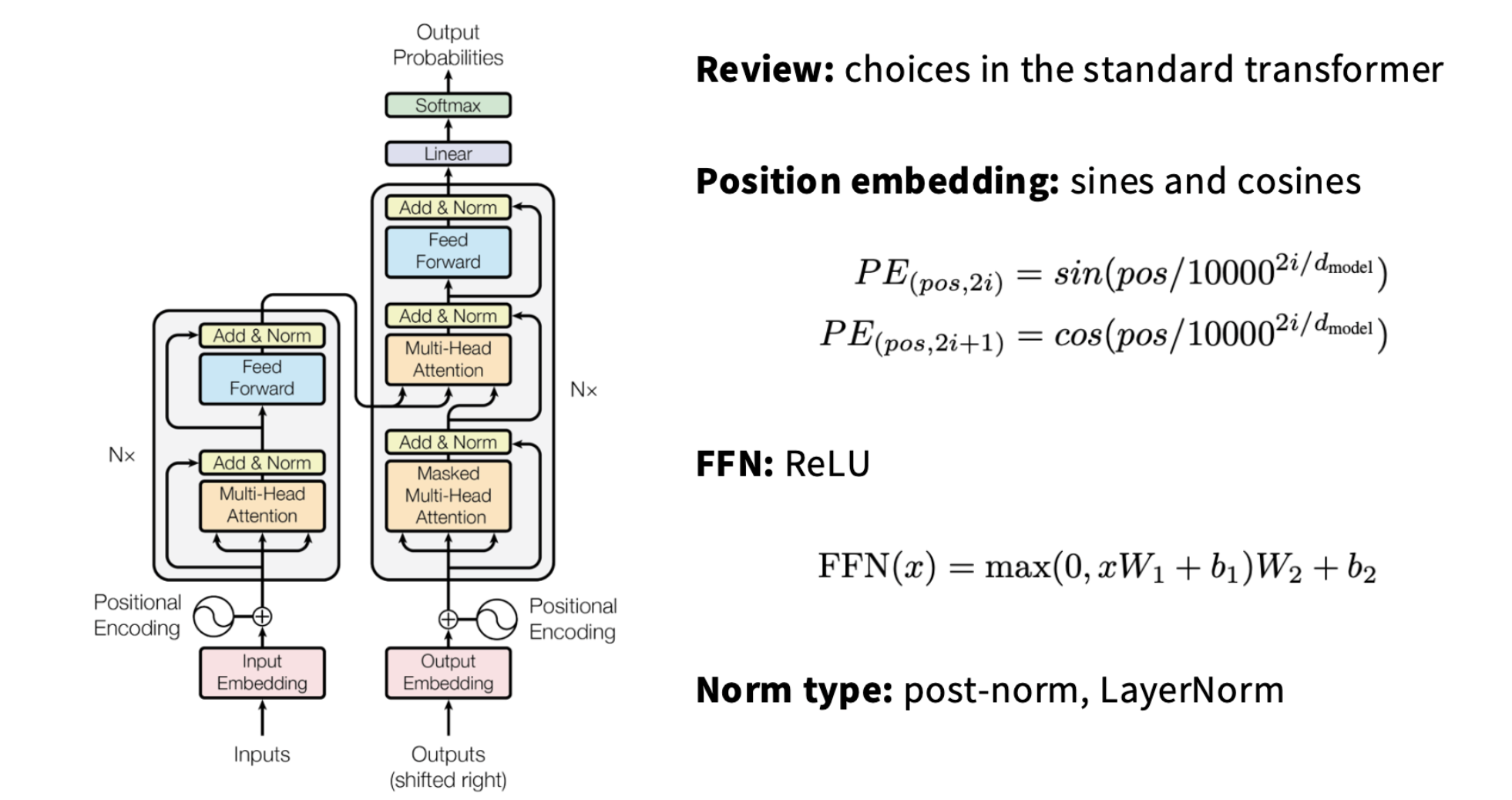
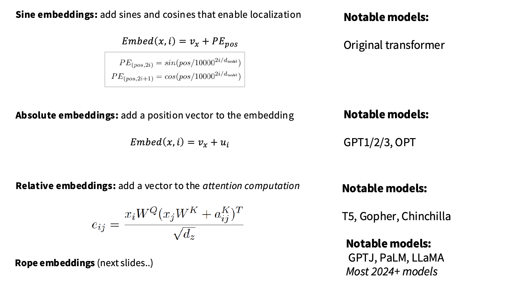
Absolute Positional Encoding

Sinusoidal Positional Encoding

Reference: [Inside Sinusoidal Position Embeddings: A Sense of Order](https://learnopencv.com/sinusoidal-position-embeddings/

The first implementation of positional encoding was the sinusoidal method, introduced by the original Transformer paper in 2017. The authors proposed a non-learned, deterministic approach using sine and cosine functions of varying wavelengths.

Their key motivation: create a position representation that enables generalization to longer sequences than those seen during training

Since our model contains no recurrence and no convolution, in order for the model to make use of the order of the sequence, we must inject some information about the relative or absolute position of the tokens in the sequence. To this end, we add “positional encodings” to the input embeddings at the bottoms of the encoder and decoder stacks. The positional encodings have the same dimension $d_{\text{model}}$ as the embeddings, so that the two can be summed. There are many choices of positional encodings, learned and fixed.

The sinusoidal position embedding $PE$ for a token at position $pos$ with embedding dimension $i$ is defined as:

\[PE(pos, 2i) = \sin(\frac{pos}{10000^{2i/d}})\] \[PE(pos, 2i+1) = \cos(\frac{pos}{10000^{2i/d}})\]

The wavelengths form a geometric progression from $2π$ to $10000 · 2π$ We chose this function because we hypothesized it would allow the model to easily learn to attend by relative positions, since for any fixed offset $k$, $PE_{pos+k}$ can be represented as a linear function of $PE_{pos}$.

We also experimented with using learned positional embeddings Convolutional Sequence to Sequence Learning instead, and found that the two versions produced nearly identical results (see Table 3 row (E)). We chose the sinusoidal version because it may allow the model to extrapolate to sequence lengths longer than the ones encountered during training.

Intuition Behind the Design

Why sine and cosine? Here’s the reasoning:

Smooth and Periodic: Allows nearby positions to have similar vectors.
Frequency Bands: Embeddings capture both coarse and fine positional changes.
Relative Position Inference: The Distance between two positions can be approximated from the inner product of their encodings.
No Parameters to Train: Reduces overfitting risk and memory usage.
Why use addition not concat?
- Why add positional embedding instead of concatenate? · Issue #1591 · tensorflow/tensor2tensor · GitHub
- Basically, positional encoding only ends up adding meaningful information to the first part of your encoding vector. The model can likely learn to reserve this for the positional encoding and include all other information about tokens with the remainder.
Why: for any fixed offset $k$, $PE_{pos+k}$ can be represented as a linear function of $PE_{pos}$
- \[PE_{pos+k} = A_k, PE_{pos}\]
- for some matrix $A_k$ that depends only on the offset $k$, not on $pos$.
- So if the positional encoding makes “move by (k)” easy to express, the model can learn relative-position behavior more easily.
- For one frequency, the encoding uses a sine/cosine pair:
- \[\sin(\omega pos), \quad \cos(\omega pos)\]
- Now look at position $pos+k$:
- \[\sin(\omega(pos+k)) = \sin(\omega pos)\cos(\omega k) + \cos(\omega pos)\sin(\omega k)\]
- \[\cos(\omega(pos+k)) = \cos(\omega pos)\cos(\omega k) - \sin(\omega pos)\sin(\omega k)\]
- This is the angle-addition formula. So the vector
- \[\begin{bmatrix} \sin(\omega(pos+k)) \\ \cos(\omega(pos+k)) \end{bmatrix}\]
- can be written as
- \[\begin{bmatrix} \cos(\omega k) & \sin(\omega k) \\ -\sin(\omega k) & \cos(\omega k) \end{bmatrix} \begin{bmatrix} \sin(\omega pos) \\ \cos(\omega pos) \end{bmatrix}\]
- That matrix depends only on $k$. So for each sine/cosine pair, shifting by $k$ is just a linear rotation.
- Across all frequencies, the full positional embedding is just all these pairs stacked together, so the whole $PE_{pos+k}$ is a linear transform of $PE_{pos}$.
Dot product of the positional embedding
- Positional encoding values (left)
- the value of the dot product of position 1000 with neighbor positions (right).
  - $PE(pos)= [\sin(\omega_1 pos),\cos(\omega_1 pos),\dots,\sin(\omega_m pos),\cos(\omega_m pos)]$ $PE(pos)\cdot PE(pos+k) = \sum_{r=1}^m \cos(\omega_r k)$
Why several cos and sin pairs?
- This design is similar to how the Fourier basis decomposes functions. Lower dimensions capture slower changes (global patterns), higher dimensions capture faster oscillations (local details).
- \[\sin(pos * 10000^{-2i/d}), \quad \cos(pos * 10000^{-2i/d})\]
  - function $\sin(\alpha x)$ has frequency $\alpha$ and period $2\pi / \alpha$
  - period: $2\pi * 10000^{2i/d}: 2\pi \to 10000* 2\pi$
  - frequency: $10000^{-2i/d}: 1 \to \frac{1}{10000}$
  - small $i$ → period short, faster oscillation
  - large $i$ → period long, slower oscillation
  - Example
    - pair 0/1: $100000=110000^0 = 1100000=1$
    - pair 2/3: $10000^{-2/8} = 10000^{-0.25} = (10^4)^{-0.25}=10^{−1}=0.1$
    - pair 4/5: $10000^{-4/8} = 10000^{-0.5} = (10^4)^{-0.5}=10^{−2}=0.01$
    - pair 6/7: $10000^{-6/8} = 10000^{-0.75} = (10^4)^{-0.75}=10^{−3}=0.001$
- Why exponential function for frequencies?
  - $pos * 10000^{-2i/d}$ evenly spaced in log space
  - position relationships are multi-scale

Animation

Pendulums swinging at different frequencies

Token position 5

Show dims 12

Slowest frequency (dim 0)

—

Fastest frequency (dim shown)

—

The snapshot captures each pendulum's angle at this position. Nearby positions look similar; distant ones diverge.

Advantages

They’re deterministic and do not need to learn
Allow the model to extrapolate to sequence lengths longer than the ones encountered during training
Relative offsets are easier to infer: easily learn to attend by relative positions, since for any fixed offset $k$, $PE_{pos+k}$ can be represented as a linear function of $PE_{pos}$.
Multi-scale position information: high frequency dimensions distinguish nearby positions; low frequency dimensions capture broader, long-range structure

Disadvantages

References: Understanding positional encoding in Transformers | Oxford Protein Informatics Group

Absolute positional encoding: Even though it contains relative structure, it is still fundamentally an absolute positional encoding added to the token embedding.
Additive encodings: To calculate attention, we take the dot product of the query and key mappings of our source and target tokens. When positional encoding is just included as part of the token embedding, we are essentially adding the relatedness of the two tokens to the positional encoding term. This means that highly related words will be given high attention scores regardless of where they are which can be problematic, especially over long sequences. The RoFormer introduced by Su et al. addresses this by making positional information multiplicative, making it easier to ignore distant tokens.
- $x_i = e_i + p_i$
- $e_i$ = word/content embedding
- $p_i$ = positional embedding
- Then attention score is based on $q_i^\top k_j$
- $(e_i + p_i)^\top (e_j + p_j) = e_i^\top e_j +e_i^\top p_j + p_i^\top e_j + p_i^\top p_j$
- $e_i^\top e_j \gg \text{position effect}$
- The first term is content similarity. If two tokens are strongly related in meaning, that term can be large. The positional terms are only extra signals, not a hard bias against long distance.
- The positional terms are only extra signals, not a hard bias against long distance.
longer lengths: Even though you can compute sinusoidal embeddings for arbitrarily long sequences, models trained on short lengths often still degrade on much longer lengths.
Not obviously optimal
Periodicity can create ambiguities: Since sine and cosine are periodic, position signals repeat in a frequency-dependent way.
Position = closeness? The second (and more fundamental) drawback of positional encoding is that it explicitly assumes that closer tokens are more important. In natural language, this is often a reasonable assumption as it relates to the natural organization of information in sentences and paragraphs. Unfortunately, other data modalities such as protein sequences have complex and non-convex positional relationships related to where the tokens lay in 3D space.
Code

Deep-ML | Problem 85

  
import numpy as np

def pos_encoding(position: int, d_model: int):
	pos = np.arange(position, dtype=np.float16)[:, np.newaxis]	
	i = np.arange(d_model, dtype=np.float16)[np.newaxis, :]
	
	angle = pos * np.power(10000, -2*(i//2)/d_model)
	pos_encoding = np.zeros((position, d_model), dtype=np.float16)
	pos_encoding[:, 0::2] = np.sin(angle[:, 0::2])
	pos_encoding[:, 1::2] = np.cos(angle[:, 1::2])
	
	return pos_encoding

Another implementation: attention-is-all-you-need-pytorch/transformer/Models.py at master · jadore801120/attention-is-all-you-need-pytorch · GitHub

  
class PositionalEncoding(nn.Module):

    def __init__(self, d_hid, n_position=200):
        super(PositionalEncoding, self).__init__()

        # Not a parameter
        self.register_buffer('pos_table', self._get_sinusoid_encoding_table(n_position, d_hid))

    def _get_sinusoid_encoding_table(self, n_position, d_hid):
        ''' Sinusoid position encoding table '''
        # TODO: make it with torch instead of numpy

        def get_position_angle_vec(position):
            return [position / np.power(10000, 2 * (hid_j // 2) / d_hid) for hid_j in range(d_hid)]

        sinusoid_table = np.array([get_position_angle_vec(pos_i) for pos_i in range(n_position)])
        sinusoid_table[:, 0::2] = np.sin(sinusoid_table[:, 0::2])  # dim 2i
        sinusoid_table[:, 1::2] = np.cos(sinusoid_table[:, 1::2])  # dim 2i+1

        return torch.FloatTensor(sinusoid_table).unsqueeze(0)

    def forward(self, x):
        return x + self.pos_table[:, :x.size(1)].clone().detach()

Learnable Positional Encoding

Advantage

Learned positional encodings adapt to data characteristics through training, potentially offering better performance when trained properly.

Disadvantage

Can’t extrapolate to longer sequences
may overfit.
increase model size since they’re part of the model parameters.
Fix to fit longer sequences
Chinese: 层次分解位置编码，让BERT可以处理超长文本

Hierarchical Decomposition of Positional Encoding More specifically, suppose we already have a set of trained absolute positional encoding vectors:

\[p_1, p_2, \dots, p_n\]

We would like to construct a new set of positional encodings:

\[q_1, q_2, \dots, q_m\]

where $m > n$

\[q_{(i-1)\times n + j} = \alpha u_i + (1 - \alpha) u_j\]

where:

$\alpha \in (0,1)$ and $\alpha \neq 0.5$ is a hyperparameter
$u_1, u_2, \dots, u_n$ are the basis vectors for the positional encoding

This formulation has a clear meaning:

Each position $(i-1)\times n + j$ is represented hierarchically as a pair $(i, j)$
The positional encodings for $i$ and $j$ are:
- $\alpha u_i$
- $(1 - \alpha) u_j$
The final encoding is the sum of the two components The constraint $\alpha \neq 0.5$ ensures that:$(i, j) \neq (j, i)$ i.e., the encoding is order-sensitive.

We want the first ( n ) positions to remain unchanged:

\[q_1 = p_1,; q_2 = p_2,; \dots,; q_n = p_n\]

This ensures compatibility with the pretrained model.

From this requirement, we can derive the basis:

\[u_i = \frac{p_i - \alpha p_1}{1 - \alpha}, \quad i = 1,2,\dots,n\]

The parameters remain $p_1, p_2, \dots, p_n$
But we can now represent up to $n^2$ positional encodings
And the first $n$ positions remain exactly the same as before

This method:

factorizes positions into two indices (i, j)
uses a compositional structure
allows extrapolation to longer sequences without retraining More details refers to the Chinese blog from the RoPE author kexue.fm/archives/7947

Code

the official GPT-2 TensorFlow implementation released by OpenAI: https://github.com/openai/gpt-2/blob/master/src/model.py
huggingface/transformers PyTorch implementation: https://github.com/huggingface/transformers/blob/main/src/transformers/models/gpt2/modeling_gpt2.py
min-GPT https://github.com/karpathy/minGPT/blob/master/mingpt/model.py

  
input = token_embedding + position_embedding

GPT-2

  
wte   # token embedding table: (vocab_size, n_embd)  
wpe   # position embedding table: (max_context, n_embd)  

wpe = tf.get_variable('wpe', [hparams.n_ctx, hparams.n_embd], initializer=tf.random_normal_initializer(stddev=0.01))
wte = tf.get_variable('wte', [hparams.n_vocab, hparams.n_embd], initializer=tf.random_normal_initializer(stddev=0.02))
past_length = 0 if past is None else tf.shape(past)[-2]
  
h = tf.gather(wte, X) + tf.gather(wpe, positions_for(X, past_length))

past_length is the number of previous tokens already cached by the model. In GPT-2 generation, the model often saves earlier attention states in past so it does not recompute them. Then:

if there is no cache yet, start positions at 0
if there is cached history, start positions at the number of past tokens

minGPT

  
wte = nn.Embedding(config.vocab_size, config.n_embd)
wpe = nn.Embedding(config.block_size, config.n_embd)
drop = nn.Dropout(config.embd_pdrop)

  
tok_emb = self.transformer.wte(idx)  
pos_emb = self.transformer.wpe(pos)  
x = self.transformer.drop(tok_emb + pos_emb)

Recursive Positional Encoding

Idea: $p_{k+1} = f(p_k)$

Similar to RNN counting behavior
Can also be modeled via ODE: $\frac{dp_t}{dt} = h(p_t, t)$

Example: FLOATER (ICML 2020)

Pros

Good extrapolation
Flexible
Cons
Less parallelizable

Relative Positional Encodings

Approach	Key Idea	Notable Implementations
Additive Distance Embeddings	Learn a vector per offset, add to q or k.	Self-Attention with Relative Position Representations Paper
Transformer-XL Bias	Shares parameters across segments to unroll histories.	Transformer-XL, XLNet
Bucketed Relative Bias	Group distances into logarithmic “buckets”.	T5, DeBERTa
ALiBi (Attention with Linear Biases)	Adds a slope × distance term – zero new tensors, constant memory.	GPT-NeoX-20B, long-context LLMs

Classical Relative Positional Encodings

Classical Design

Relative Positional Encodings origins from Google paper Self-Attention with Relative Position Representations

In paper:

We propose an extension to self-attention to consider the pairwise relationships between input elements. In this sense, we model the input as a labeled, directed, fully-connected graph.

Edge Representations in Attention The edge between input elements $x_i$ and $x_j$ is represented by vectors: $a^V_{ij}, ; a^K_{ij} \in \mathbb{R}^{d_a}$

The motivation for learning two distinct edge representations is that:

$a^V_{ij}$ is suitable for use in value aggregation
- \[z_i = \sum_{j=1}^{n} \alpha_{ij} \left( x_j W^V + {\color{blue}a^V_{ij}} \right)\]
- Standard attention: uses only $x_j W^V$
- Now: inject edge information via $a^V_{ij}$
- “This extension is presumably important for tasks where information about the edge types selected by a given attention head is useful to downstream encoder or decoder layers. However, as explored in 4.3, this may not be necessary for machine translation.”
$a^K_{ij}$ is suitable for use in attention score computation
- \[e_{ij} =\frac{ x_i W^Q \left( x_j W^K + {\color{blue}a^K_{ij}} \right)^\top}{\sqrt{d_z}}\]
- Standard attention: $x_i W^Q \cdot x_j W^K$
- Now: $x_i W^Q \cdot (x_j W^K + a^K_{ij})$
- Edge information directly affects attention weights
$x_j W^K + a^K_{ij}, \quad x_j W^V + a^V_{ij}$
- The primary motivation for using simple addition to incorporate edge representations is to enable an efficient implementation.
These representations can be shared across attention heads. We use: $d_a = d_z$ This avoids requiring additional linear transformations.

Another Explanation

There is another way to understand it, according to JianLin Su’s Chinese Blog It is generally believed that relative positional encoding is inspired by absolute positional encoding.

Consider the standard attention mechanism with absolute positional encoding:

\[\begin{cases} q_i = (x_i + p_i) W_Q \\ k_j = (x_j + p_j) W_K \\ v_j = (x_j + p_j) W_V \\ a_{i,j} = \text{softmax}_j(q_i k_j^\top) \\ o_i = \sum_j a_{i,j} v_j \end{cases}\]

The softmax is applied over dimension $j$
All vectors are treated as row vectors

Expand the Attention Score $q_i k_j^\top = (x_i + \bcancel{p_i}) W_Q W_K^\top (x_j + p_j)^\top = (x_i W_Q + \bcancel{p_i W_Q})(W_K^\top x_j^\top + {\color{blue}W_K^\top p_j^\top})$

To introduce relative positional information, Google proposed:

Remove positional term from the query side $p_i$
Replace $p_j W_K$ with a pairwise relative position embedding $R^K_{i,j}$

New Attention Score $a_{i,j} = \text{softmax}\left(x_i W_Q (x_j W_K + {\color{blue}R^K_{i,j}})^\top \right)$

Also replace absolute position with relative in $o_i$ $o_i = \sum_j a_{i,j} (x_j W_V + p_j W_V)$

Become $o_i = \sum_j a_{i,j} (x_j W_V + {\color{blue}R^V_{i,j}})$

Defining Relative Position

Instead of depending on absolute indices $(i, j)$, define $R^K_{i,j}, R^V_{i,j}$ depend only on $(i - j)$

Distance-based Encoding with Clipping

$\begin{align} R^K_{i,j} &= p^K_{\text{clip}(j-i, k)}\\ R^V_{i,j} &= p^V_{\text{clip}(j-i, k)} \\ \text{clip}(x, k) &= max(-k, min(k, x)) \end{align}$

For linear sequences, edges can capture information about the relative position differences between input elements. The maximum relative position we consider is clipped to a maximum absolute value of $k$. We hypothesized that precise relative position information is not useful beyond a certain distance. Clipping the maximum distance also enables the model to generalize to sequence lengths not seen during training. Therefore, we consider $2k + 1$ unique edge labels.

Key Idea

Only depend on relative distance $i - j$
Use clipping to limit range:
- Handles arbitrarily long sequences
- Keeps parameter size finite

This design allows:

A finite set of embeddings $p^K = (p_{-k}^K, …, p_k^K), p^V= (p_{-k}^V, …, p_k^V)$
To represent arbitrary sequence lengths
Works whether embeddings are:
- learned
- sinusoidal

Code

  
import torch.nn as nn

class RelativePositionalEncoding(nn.Module):
    def __init__(self, max_relative_position, d_model):
        super().__init__()
        self.max_relative_position = max_relative_position
        self.relative_attention_bias = nn.Parameter(
            torch.randn(2 * max_relative_position + 1, d_model)
        )
    
    def forward(self, length):
        context_position = torch.arange(length, dtype=torch.long)[:, None]
        memory_position = torch.arange(length, dtype=torch.long)[None, :]
        relative_position = memory_position - context_position
        relative_position_bucket = relative_position + self.max_relative_position
        return self.relative_attention_bias[relative_position_bucket]

The relative_position matrix has shape (length, length), with each element representing the relative position between tokens 𝑖 and 𝑗. This is computed by subtracting an 𝑁 ×1 matrix context_position from a 1 ×𝑁 matrix memory_position. The relative_position_bucket shifts values to be non-negative, and position encoding vectors are looked up from the relative_attention_bias tensor.

Relative positional encodings naturally handle variable-length sequences and work well for tasks like translation, making them the choice for models like T5.

Attention with Linear Bias (ALiBi) is a related approach that adds a bias matrix to attention scores instead of manipulating the input sequence. In the code above, you see that relative_positon_bucket is used to look up a sequence of vectors as the positional encoding, which is then added to the input sequence in the attention module. In ALiBi, the input sequence are used directly in calculating the attention score. But afterwards, the matrix of relative_positon_bucket is scaled and added to the attention score matrix before proceeding to the softmax operation. The scaling factor in ALiBi is computed as $𝑚ℎ =1/2^{8⁢ℎ⁡/𝐻}$, where $ℎ$ is the head index and $𝐻$ is the total number of attention heads.

XLNET Relative Positional Encoding

[1901.02860] Transformer-XL: Attentive Language Models Beyond a Fixed-Length Context The following terminology follows the JianLin Su’s Chinese Blog

Derived from full expansion:

\[q_i k_j^\top =x_i W_Q W_K^\top x_j^\top - x_i W_Q W_K^\top p_j^\top - p_i W_Q W_K^\top x_j^\top - p_i W_Q W_K^\top p_j^\top\]

Classical Relative Positional Encoding
- $p_i \to 0$
- $p_j W_K \to R^K_{i,j}$, and clip $R^K_{i,j} = p^K_{\text{clip}(j-i, k)}$
XLNET Relative Positional Encoding
- $p_i \rightarrow u, v$ (learnable)
- $p_j \rightarrow R_{i-j}$, sinusoidal relative encoding

\[x_i W_Q W_K^\top x_j^\top - x_i W_Q W_K^\top {\color{blue}R_{i-j}^\top} - {\color{teal}u} W_Q W_K^\top x_j^\top - {\color{teal}v} W_Q W_K^\top {\color{blue}R_{i-j}^\top}\]

XLNET Relative Positional Encoding Final Form
- $p_i \rightarrow u, v$ (learnable); and then $p_iW_Q \rightarrow u, v$ (learnable);
- $p_j \rightarrow R_{i-j}$, sinusoidal relative encoding, No Clipping
  - $R_{i−j}$ may not have the same embedding space with $x_j$
  - So replace $W_K^\top R_{i−j}^\top \to {\color{magenta}W_{K,R}^\top} R_{i−j}^\top$

\[x_i W_Q W_K^\top x_j^\top - x_i W_Q {\color{magenta}W_{K,R}^\top} {\color{blue}R_{i-j}^\top} - {\color{teal}u} W_K^\top x_j^\top - {\color{teal}v} {\color{magenta}W_{K,R}^\top} {\color{blue}R_{i-j}^\top }\]

Removes positional term from value:

\[o_i = \sum_j a_{i,j} x_j W_V\]

Subsequent studies prefer incorporating relative positional embeddings into the attention matrix rather than the value vector.

T5 Relative Position Embedding

The T5 model (from [1910.10683] Exploring the Limits of Transfer Learning with a Unified Text-to-Text Transformer) uses a simpler relative positional encoding.

\[q_i k_j^\top = x_i W_Q W_K^\top x_j^\top - x_i W_Q W_K^\top p_j^\top - p_i W_Q W_K^\top x_j^\top - p_i W_Q W_K^\top p_j^\top\]

This can be interpreted as four components:

input–input
input–position
position–input
position–position

Key Idea: Decouple Content and Position

If we assume: content and positional information should be independent, then we remove cross terms:
- ~~input–position~~
- ~~position–input~~

Then we have Simplified Form (T5) only including input–input and position–position $x_i W_Q W_K^\top x_j^\top + {\color{blue}\beta_{i,j}}$ where:

$\beta_{i,j}$ is a learnable scalar bias
depends only on $(i, j)$

T5 RPE is just adding a bias term to the attention matrix

Similar Ideas: [2006.15595] Rethinking Positional Encoding in Language Pre-training
Relative Position Bucketing

Instead of directly using $\beta_{i,j}$ as a function of $i-j$ with clipping, T5 applies a mapping with buckets: $pos(i - j) \rightarrow pos(f(i - j))$

small distances → fine-grained buckets
large distances → coarse buckets

Example:

distance: 0–7, bucket: unique
8–11: shared
larger: increasingly coarse

DeBERTa Positional Encoding

[2006.03654] DeBERTa: Decoding-enhanced BERT with Disentangled Attention

Key Difference vs T5

T5 keeps position–position (remove position-input and input-position)
DeBERTa keeps input–position and position–input (remove position-position)
- $R_{i,j}$ also need clipping

\[q_i k_j^\top = x_i W_Q W_K^\top x_j^\top + x_i W_Q W_K^\top {\color{blue}R_{i,j}^\top} + {\color{blue}R_{j,i}} W_Q W_K^\top x_j^\top\]

Architectural Insight

DeBERTa separates:

relative position (early layers)
absolute position (later layers) Example in MLM Pre-train Base:
first 11 layers → relative (“Encoder” not classical encoder)
last 2 layers → add absolute (“Decoder / Enhanced Mask Decoder (EMD)” not classical)

ALiBi: Attention with Linear Biases

[2108.12409] Train Short, Test Long: Attention with Linear Biases Enables Input Length Extrapolation

Adds a slope × distance term – zero new tensors, constant memory.

Compares to T5

\[\text{score}_{ij}=\frac{q_i k_j^\top}{\sqrt{d}} + \text{position\_bias}(i,j)\]

T5 uses a learned bias based on the relative distance between query position (i) and key position $j$.

\[\text{score}_{ij}=\frac{q_i k_j^\top}{\sqrt{d}} + b_{\text{bucket}(i-j)}\]

Where:

$i-j$ is the relative distance
distances are mapped into buckets:
- small distances get fine resolution, large distances are grouped into coarser buckets
each bucket has a learned scalar bias
usually each attention head has its own learned bias table

ALiBi uses a fixed linear penalty:

\[\text{score}_{ij}=\frac{q_i k_j^\top}{\sqrt{d}} - m_h(i-j)\]

for causal attention.

Where

$m_h$ is a fixed slope for head $h$
farther tokens get penalized more
no learned bucket table is needed

ALiBi hardcodes the prior:

closer tokens should usually matter more
farther tokens should get lower attention unless content strongly overcomes the penalty

Benefits

This is simple and not learned.
ALiBi often extrapolates better to longer lengths because the rule is simple: just keep extending the linear penalty

Other Positional Encoding Methods

CNN-style (Implicit Position Encoding)

CNNs typically do not use explicit position encoding.

Key finding

From [2001.08248] How Much Position Information Do Convolutional Neural Networks Encode? Interestingly, the paper shows that:

positional information comes from zero padding

Because padding introduces artificial boundaries, the model can implicitly learn: $\text{position} \approx \text{distance to padding boundary}$ In other words, CNNs are effectively learning: relative distance between the current location and the padded edges

This positional awareness relies on: locality of CNNs
- Convolutions operate on local neighborhoods
- Boundary effects propagate inward layer by layer
Why this does NOT apply to Transformers
- Attention is: $\text{global} + \text{no spatial prior}$
- No inherent notion of locality
- No boundary signal like padding
- Cannot infer position implicitly
why ViT-style network still needs positional encoding even though it uses patches
- once patches become tokens, spatial structure is lost.

Complex Order Positional Encoding

From [1912.12333] Encoding word order in complex embeddings

\[\big[r_{j,1} e^{i(\omega_{j,1} k + \theta_{j,1})}, \dots, r_{j,d} e^{i(\omega_{j,d} k + \theta_{j,d})}\big]\]

$\begin{align} r_j &= [r_{j,1}, \dots, r_{j,d}], \\ \omega_j &= [\omega_{j,1}, \dots, \omega_{j,d}], \\ \theta_j &= [\theta_{j,1}, \dots, \theta_{j,d}] \end{align}$

$i$ is imaginary unit
$j$ denotes a token(word)
$k$ denotes the position of the token
Each token has three pair of embeddings
Encoding uses complex numbers
Entire Transformer becomes complex-valued

RoPE: Rotary Positional Embeddings

RoPE

Original Paper: ROFORMER: ENHANCED TRANSFORMER WITH ROTARYPOSITION EMBEDDING
Original Code: GitHub - ZhuiyiTechnology/roformer: Rotary Transformer · GitHub
PyTorch version: GitHub - JunnYu/RoFormer_pytorch: RoFormer V1 & V2 pytorch · GitHub
Blog: Rotary Embeddings: A Relative Revolution | EleutherAI Blog
Chinese Blog: kexue.fm/archives/8265
RoPE ViT

What is RoPE

Most model user RoPE Now
apply a 2D rotation to every pair of dimensions.
- For one pair: [x1, x2], a rotation by angle θ is: [x1 cosθ - x2 sinθ, x1 sinθ + x2 cosθ]
- Now look at this rewrite:[x1, x2] * cosθ + [-x2, x1] * sinθ
Instead of adding, it applies a rotation matrix to the query and key vectors before the dot-product attention
- the dot product between two rotated vectors reflects their relative distance, RoPE gives native access to relative position without learning or storing extra embeddings.

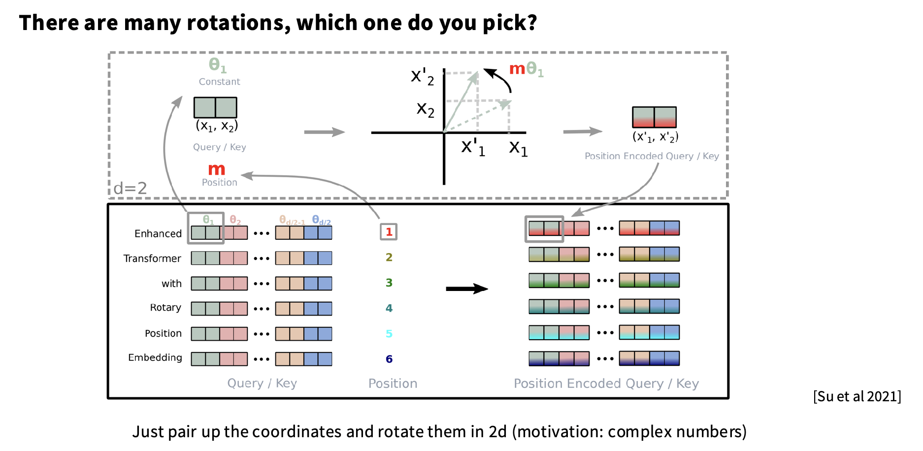
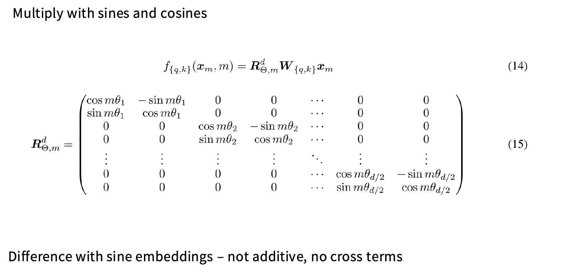
The rotation matrix $\mathbf{R}_𝑚$ geometrically rotates the 2D input vector by an angle $𝑚⁢𝜃_𝑖$
The transpose $\mathbf{R}^T_𝑚$ = $\mathbf{R}^{−1}_𝑚$
represents reverse rotation.
Hence the relative positions can be easily computed as $\mathbf{R}_{𝑚−𝑛} =\mathbf{R}_𝑚𝐑^⊤_𝑛$
It can extrapolate to longer sequences due to the geometric progression of angles
Since $cos^2⁡𝑡 +sin^2⁡𝑡 =1$, RoPE preserves vector norms of $\mathbf{x}_m$, aiding training stability

How to Design RoPE

In RoPE (Rotary Positional Encoding), the starting point is:

Use absolute positional encoding to achieve relative positional effects

Theoretically elegant
Practically useful: Can extend to linear attention

We define a function $f(\cdot, m)$ that injects position into vectors:

\[\tilde{q}_m = f(q, m), \quad \tilde{k}_n = f(k, n)\]

$q$, $k$: original query and key vectors
$\tilde{q}_m$, $\tilde{k}_n$: position-aware vectors
$f(\cdot, m)$: injects absolute position $m$

Desired Property Attention relies on inner products: $\langle q, k \rangle$ We want: $\textcolor{blue}{\text{the inner product to encode relative position} \quad m - n}$

\[\langle f(q, m), f(k, n) \rangle = g(q, k, m - n)\]

Left side: uses absolute positions
Right side: depends only on relative distance
Initial Conditions: $f(q, 0) = q, f(k, 0) = k$.
- At position 0 → no transformation.
- Ensures consistency with original vectors

Problems

Failure mode	Root cause	Observable symptom
Phase-shift drift	Using the original training slope (base = 10,000) on a much longer window causes high-frequency pairs to spin too quickly, making it difficult for attention to maintain fine detail.	Sudden loss of syntactic coherence or repeated text after ~8k–16k tokens.
Numerical precision	For very large `p`, floating-point rounding collapses `sin θ` ≈ `sin(θ+ε)`, especially in fp16/bfloat16.	Gradient vanishing in fine-tune; attention logits become noisy for far-right tokens.
Kernel/cache mismatch	Some Flash-Attention & KV-cache variants implicitly assume angle ≤ π; when scaled to 256 k via RoPE-linear, we violate that bound.	Model emits garbage once the cache slides beyond a few segments.
Training–inference distribution gap	Model only saw 4k tokens; at 32k, it has never learned to chain-reason across segments.	Quality degrades smoothly even if positional math is correct.
Modal mis-alignment in VLMs	Text RoPE (1-D) reused for image patches (2-D) causes anisotropy.	Model favours horizontal relations; diagonal relations are misattended.
Cross-head interference	All heads share identical clock set; certain heads “lock-on” to harmonics, starving others of positional variance.	Sharp head-wise sparsity in attention heat-maps; instability during SFT.

No learned adaptation – Being parameter-free, RoPE can’t specialise to domain-specific structures (e.g., XML trees) the way a learned RPE could.
Axis coupling in 2-D/3-D inputs – Standard 1-D RoPE treats flattened patch order; we need Axial-RoPE or 2-D RoPE to remove artefacts.
Streaming constraints – At extremely long contexts, we still pay O(L²) memory/time unless combined with sliding-window masks or memory-computation hybrids (LongLoRA, Ring-Attention).
Precision cliffs – In mixed-precision inference, large angles lead to sin⁡, cos⁡ values that differ by < ε of fp16, effectively collapsing several high-freq clocks to the same vector (“angle saturation”).

RoPE’s practical weak spots come much earlier than its theoretical 62 k-token slow-clock wrap-around. Real issues include phase drift of the fast clocks, floating-point precision, training-window mismatch, and modality-specific geometry. Modern scaling tricks or hybrid encodings tackle those problems directly; simply enlarging d (and thus marginally bumping the slowest wavelength) does little to cure them.

Code

  
import numpy as np

def apply_rope(x: np.ndarray, positions: np.ndarray, base: float = 10000.0) -> np.ndarray:
	"""
	Args:
	x: Array of shape (seq_len, d), where d is even.
	positions: Array of shape (seq_len,) with integer positions.
	base: Base used to compute rotation frequencies.
	Returns:
	Array of shape (seq_len, d) with RoPE applied.
	"""
	if x.ndim != 2:
		raise ValueError("x must have shape (seq_len, d)")
	if positions.ndim != 1:
		raise ValueError("positions must have shape (seq_len,)")
	if x.shape[0] != positions.shape[0]:
		raise ValueError("seq_len of x and positions must match")
	
	if x.shape[1] % 2 != 0:
		raise ValueError("embedding dimension d must be even")
	
	seq_len, d = x.shape
	half_d = d // 2
	
	# Frequencies for each pair of dimensions
	pair_idx = np.arange(half_d, dtype=np.float64)
	freqs = base ** (- 2.0 * pair_idx / d) # shape: (half_d,)
	
	# Rotation angles for each position and pair
	angles = positions[:, None].astype(np.float64) * freqs[None, :] # (seq_len, half_d)
	
	cos = np.cos(angles)
	sin = np.sin(angles)
	
	# Split into even/odd pairs
	x_even = x[:, 0::2].astype(np.float64) # (seq_len, half_d)
	x_odd = x[:, 1::2].astype(np.float64) # (seq_len, half_d)
	
	# Apply 2D rotation to each pair
	out_even = x_even * cos - x_odd * sin
	out_odd = x_even * sin + x_odd * cos
	
	# Interleave back to shape (seq_len, d)
	out = np.empty((seq_len, d), dtype=np.float64)
	out[:, 0::2] = out_even
	out[:, 1::2] = out_odd
	return out.astype(x.dtype, copy=False)

  
import numpy as np
def rotate_half(x: np.ndarray) -> np.ndarray:
	x1 = x[..., ::2]
	x2 = x[..., 1::2]
	y = np.stack((-x2, x1), axis=-1)
	return y.reshape(x.shape)
	
def rotate_half(x):  
	y = np.empty_like(x)  
	y[..., 0::2] = -x[..., 1::2]  
	y[..., 1::2] = x[..., 0::2]  
	return y

def apply_rope(x: np.ndarray, positions: np.ndarray, base: float = 10000.0) -> np.ndarray:
	"""
	Args:
	x: Array of shape (seq_len, d), where d is even.
	positions: Array of shape (seq_len,) with integer positions.
	base: Base used to compute rotation frequencies.
	Returns:
	Array of shape (seq_len, d) with RoPE applied.
	"""

	seq_len, d = x.shape
	assert d % 2 == 0
	half = d // 2
	pair_idx = np.arange(half, dtype=np.float32)
	
	# frequency for each dimension pair
	freqs = base ** (-2.0 * pair_idx / d) # (half,)
	
	# angle for each token position and each pair
	angles = positions[:, None].astype(np.float32) * freqs[None, :] # (seq_len, half)
	
	# expand so each angle is used for both dims in a pair
	cos = np.repeat(np.cos(angles), 2, axis=-1) # (seq_len, d)
	sin = np.repeat(np.sin(angles), 2, axis=-1) # (seq_len, d)
	
	x_rot = x * cos + rotate_half(x) * sin
	
	return x_rot

pseudo code

  
sinusoidal_pos.shape = [1, seq_len, hidden_size] # Sinusoidal position embeddings
qw.shape = [batch_size, seq_len, num_heads, hidden_size]  # query hiddens
kw.shape = [batch_size, seq_len, num_heads, hidden_size]  # key hiddens

cos_pos = repeat_elements(sinusoidal_pos[..., None, 1::2], rep=2, axis=-1)
sin_pos = repeat_elements(sinusoidal_pos[..., None, ::2], rep=2, axis=-1)
qw2 = stack([-qw[..., 1::2], qw[..., ::2]], 4)
qw2 = reshape(qw2, shape(qw))
qw = qw * cos_pos + qw2 * sin_pos
kw2 = K.stack([-kw[..., 1::2], kw[..., ::2]], 4)
kw2 = K.reshape(kw2, K.shape(kw))
kw = kw * cos_pos + kw2 * sin_pos

# Attention
a = tf.einsum('bjhd,bkhd->bhjk', qw, kw)

NoPE: No Positional Embeddings

Reference: No Positional Embeddings (NoPE) | Sebastian Raschka, PhD Paper:

[2404.12224] Length Generalization of Causal Transformers without Position Encoding
[2305.19466] The Impact of Positional Encoding on Length Generalization in Transformers
What NoPE is
NoPE means not adding any explicit positional encoding to attention layers: no learned absolute embeddings, no sinusoidal embeddings, no RoPE. Queries and keys are used without position injection.
Why this can still work
Even without explicit position embeddings, an autoregressive transformer still has the causal mask, so token at position $t$ can only attend to tokens at positions $≤t$. That gives the model an implicit directional notion of order. The claim is that training can learn to exploit this structure.
Main motivation
The big appeal is length generalization. With RoPE or other explicit positional schemes, the model may run into trouble at sequence lengths beyond what it saw in training. NoPE avoids that “unseen position / unseen rotation angle” issue by construction, since there is no explicit position signal to extrapolate.

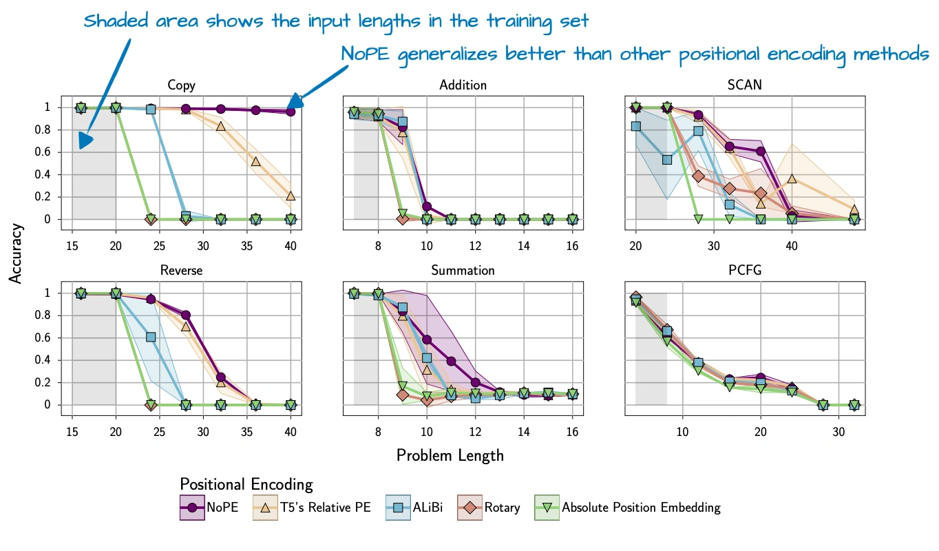The original NoPE motivation was stronger length generalization when explicit positional encodings are removed. (Original source: NoPE paper.)

How it appears in modern models

NoPE as a real design choice in newer LLMs, not just a theory idea. Examples mentioned in No Positional Embeddings (NoPE) | Sebastian Raschka, PhD

SmolLM3, which experiments with NoPE layers.
Kimi Linear, which uses NoPE in its MLA/global attention layers, while other blocks handle sequence structure differently.

Practical tradeoff
The article’s framing is not “NoPE is always better than RoPE.” It is more:

Recent hybrid and long-context models often keep RoPE in local or sliding-window attention layers while dropping it in selected global-attention layers.
but NoPE is a useful alternative when long-context robustness or simplicity is attractive.

iRoPE: “interleaved” attention & “infinite” context length

The Llama 4 herd: The beginning of a new era of natively multimodal AI innovation llama-models/models/llama4/model.py at main · meta-llama/llama-models · GitHub

Code

Transformer Block

_nope_layer_interval_ : 4

  
class TransformerBlock(nn.Module):
    def __init__(self, layer_id: int, args: ModelArgs):
        super().__init__()
        self.n_heads = args.n_heads
        self.dim = args.dim
        self.head_dim = args.dim // args.n_heads if args.head_dim is None else args.head_dim

        self.is_nope_layer = args.nope_layer_interval is not None and (layer_id + 1) % args.nope_layer_interval == 0

        use_rope = not self.is_nope_layer
        use_qk_norm = args.use_qk_norm and not self.is_nope_layer

        self.attention = Attention(args, use_rope=use_rope, use_qk_norm=use_qk_norm)

Attention Forward

Project x into Q, K, V
Reshape into heads
Optionally apply RoPE to Q, K
Optionally apply QK norm (rmsnorm)
- xq = rmsnorm(xq, self.norm_eps)
- xk = rmsnorm(xk, self.norm_eps)
- if Q/K norms vary too much, logits can become too sharp or unstable
For NoPE layers, optionally do attention temperature tuning
- temperature tuning (https://arxiv.org/abs/2501.19399) to NoPE layers
  - small positions: scale stays close to 1;
  - long positions: scale grows slowly, using a log-based rule
- Without RoPE, the model may need help as context gets very long. This mechanism changes the sharpness of attention as sequence position grows, but tries not to disturb short contexts much:
  - floor((pos+1)/floor_scale) means nothing changes until position passes a chunk boundary
  - then log(...)+1 increases slowly
  - so short context is mostly unaffected, very long context gets stronger scaling.
- This is not adding positional information in the usual sense. It is changing the magnitude of the queries by position, which changes attention sharpness. So it is more like inference-time temperature control than positional encoding
Write new keys/values into the KV cache
- self.cache_k[:bsz, start_pos : start_pos + seqlen] = xk
- self.cache_v[:bsz, start_pos : start_pos + seqlen] = xv
Attend from current queries to all cached keys/values
Merge heads and project back out.

  
    def forward(
        self,
        x: torch.Tensor,
        start_pos: int,
        freqs_cis: torch.Tensor,
        mask: Optional[torch.Tensor] = None,
    ):
        bsz, seqlen, _ = x.shape
        xq, xk, xv = self.wq(x), self.wk(x), self.wv(x)

        xq = xq.view(bsz, seqlen, self.n_local_heads, self.head_dim)
        xk = xk.view(bsz, seqlen, self.n_local_kv_heads, self.head_dim)
        xv = xv.view(bsz, seqlen, self.n_local_kv_heads, self.head_dim)

        if self.use_rope:
            xq, xk = apply_rotary_emb(xq, xk, freqs_cis=freqs_cis)

        if self.use_qk_norm:
            xq = rmsnorm(xq, self.norm_eps)
            xk = rmsnorm(xk, self.norm_eps)

        # We are applying temperature tuning (https://arxiv.org/abs/2501.19399) to NoPE layers, where
        # the inference-time temperature tuning function is customized to not affect short context
        # while working at very long context
        if self.attn_temperature_tuning and not self.use_rope:
            seq_positions = torch.arange(start_pos, start_pos + seqlen, device=xq.device, dtype=torch.float32)
            attn_scales = torch.log(torch.floor((seq_positions + 1.0) / self.floor_scale) + 1.0) * self.attn_scale + 1.0

            # reshape for broadcasting [seqlen] -> [1, seqlen, 1, 1]
            attn_scales = attn_scales.view(1, seqlen, 1, 1)
            xq = xq * attn_scales

        self.cache_k = self.cache_k.to(xq)
        self.cache_v = self.cache_v.to(xq)

        self.cache_k[:bsz, start_pos : start_pos + seqlen] = xk
        self.cache_v[:bsz, start_pos : start_pos + seqlen] = xv

        xk = self.cache_k[:bsz, : start_pos + seqlen]
        xv = self.cache_v[:bsz, : start_pos + seqlen]

        xq, xk, xv = [t.transpose(1, 2) for t in (xq, xk, xv)]

        xk = xk.repeat_interleave(self.n_rep, dim=1)
        xv = xv.repeat_interleave(self.n_rep, dim=1)

        attn_output = F.scaled_dot_product_attention(xq, xk, xv, attn_mask=mask, dropout_p=0.0)
        attn_output = attn_output.transpose(1, 2).contiguous().view(bsz, seqlen, -1)
        output = self.wo(attn_output)
        return output

Vision Transformer (ViT)

[2010.11929] An Image is Worth 16x16 Words: Transformers for Image Recognition at Scale

Position embeddings are added to the patch embeddings to retain positional information. We use standard learnable 1D position embeddings, since we have not observed significant performance gains from using more advanced 2D-aware position embeddings (Appendix D.4). The resulting sequence of embedding vectors serves as input to the encoder.

Appendix D.4 compares more 2010.11929 page:16.54

Pos. Emb.	Default/Stem	Every Layer	Every Layer-Shared
No Pos. Emb.	0.61382	N/A	N/A
1-D Pos. Emb.	0.64206	0.63964	0.64292
2-D Pos. Emb.	0.64001	0.64046	0.64022
Rel. Pos. Emb.	0.64032	N/A	N/A

Caption: Results of the ablation study on positional embeddings with ViT-B/16 model evaluated on ImageNet 5-shot linear.

References

Transformer

Transformer Attention

This post is licensed under CC BY 4.0 by the author.

Why need positional encoding

Absolute Positional Encoding

Sinusoidal Positional Encoding

Intuition Behind the Design

Animation

Advantages

Disadvantages

Code

Learnable Positional Encoding

Advantage

Disadvantage

Fix to fit longer sequences

Code

Recursive Positional Encoding

Pros

Cons

Relative Positional Encodings

Classical Relative Positional Encodings

Classical Design

Another Explanation

Distance-based Encoding with Clipping

Code

XLNET Relative Positional Encoding

T5 Relative Position Embedding

Key Idea: Decouple Content and Position

Relative Position Bucketing

DeBERTa Positional Encoding

Key Difference vs T5

Architectural Insight

ALiBi: Attention with Linear Biases

Compares to T5

Other Positional Encoding Methods

CNN-style (Implicit Position Encoding)

Key finding

Complex Order Positional Encoding

RoPE: Rotary Positional Embeddings

RoPE

What is RoPE

How to Design RoPE

Problems

Code

NoPE: No Positional Embeddings

What NoPE is

Why this can still work

Main motivation

How it appears in modern models

iRoPE: “interleaved” attention & “infinite” context length

Code

Transformer Block

Attention Forward

Vision-Related (To Be Cont.)

Vision Transformer (ViT)

References

Trending Tags