Vision Transformer (ViT)
Paper & Code
- Paper: [2010.11929] An Image is Worth 16x16 Words: Transformers for Image Recognition at Scale
- Code: GitHub - google-research/vision_transformer · GitHub
- PyTorch Official:
- HuggingFace:
Overview
The Vision Transformer (ViT) model was proposed in An Image is Worth 16x16 Words: Transformers for Image Recognition at Scale by Alexey Dosovitskiy, Lucas Beyer, Alexander Kolesnikov, Dirk Weissenborn, Xiaohua Zhai, Thomas Unterthiner, Mostafa Dehghani, Matthias Minderer, Georg Heigold, Sylvain Gelly, Jakob Uszkoreit, Neil Houlsby. It’s the first paper that successfully trains a Transformer encoder on ImageNet, attaining very good results compared to familiar convolutional architectures. (From HuggingFace)
Paper Abstract: While the Transformer architecture has become the de-facto standard for natural language processing tasks, its applications to computer vision remain limited. In vision, attention is either applied in conjunction with convolutional networks, or used to replace certain components of convolutional networks while keeping their overall structure in place. We show that this reliance on CNNs is not necessary and a pure transformer applied directly to sequences of image patches can perform very well on image classification tasks. When pre-trained on large amounts of data and transferred to multiple mid-sized or small image recognition benchmarks (ImageNet, CIFAR-100, VTAB, etc.), Vision Transformer (ViT) attains excellent results compared to state-of-the-art convolutional networks while requiring substantially fewer computational resources to train.
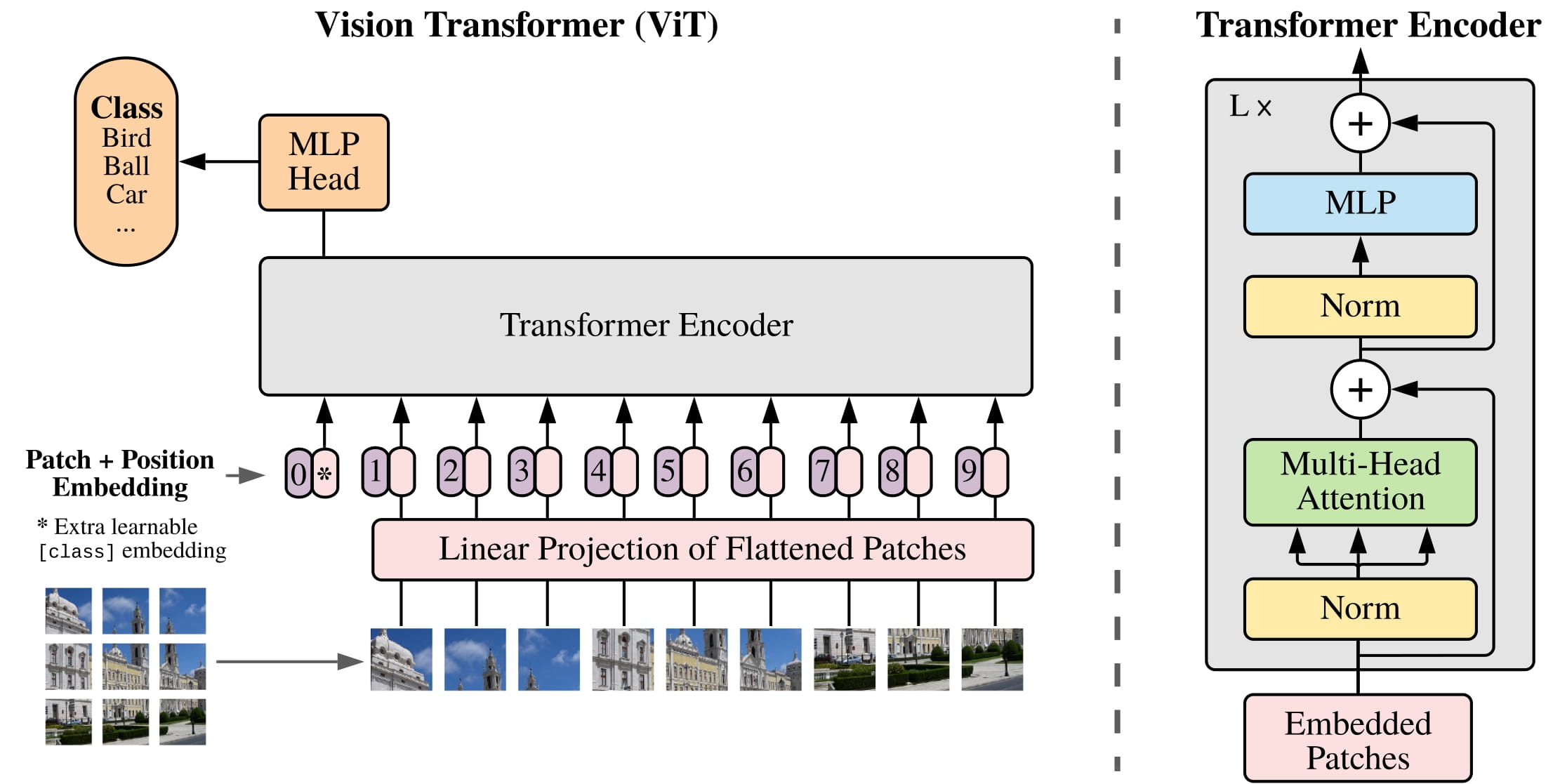 ViT architecture. Taken from the original paper.
All the quoted parts in this post is from original paper.
Model
HuggingFace - google/vit-base-patch16-224
Model Summary
1
2
3
4
5
from transformers import ViTForImageClassification
import torch
import numpy as np

model = ViTForImageClassification.from_pretrained("google/vit-base-patch16-224")
1
2
3
4
5
6
7
8
9
10
11
12
13
14
15
16
17
18
19
20
21
22
23
24
25
26
27
28
29
30
31
32
33
34
35
36
37
38
39
ViTForImageClassification(
  (vit): ViTModel(
    (embeddings): ViTEmbeddings(
      (patch_embeddings): ViTPatchEmbeddings(
        (projection): Conv2d(3, 768, kernel_size=(16, 16), stride=(16, 16))
      )
      (dropout): Dropout(p=0.0, inplace=False)
    )
    (encoder): ViTEncoder(
      (layer): ModuleList(
        (0-11): 12 x ViTLayer(
          (attention): ViTAttention(
            (attention): ViTSelfAttention(
              (query): Linear(in_features=768, out_features=768, bias=True)
              (key): Linear(in_features=768, out_features=768, bias=True)
              (value): Linear(in_features=768, out_features=768, bias=True)
            )
            (output): ViTSelfOutput(
              (dense): Linear(in_features=768, out_features=768, bias=True)
              (dropout): Dropout(p=0.0, inplace=False)
            )
          )
          (intermediate): ViTIntermediate(
            (dense): Linear(in_features=768, out_features=3072, bias=True)
            (intermediate_act_fn): GELUActivation()
          )
          (output): ViTOutput(
            (dense): Linear(in_features=3072, out_features=768, bias=True)
            (dropout): Dropout(p=0.0, inplace=False)
          )
          (layernorm_before): LayerNorm((768,), eps=1e-12, elementwise_affine=True)
          (layernorm_after): LayerNorm((768,), eps=1e-12, elementwise_affine=True)
        )
      )
    )
    (layernorm): LayerNorm((768,), eps=1e-12, elementwise_affine=True)
  )
  (classifier): Linear(in_features=768, out_features=1000, bias=True)
)
ViTModel
1
2
3
4
5
6
7
8
self.embeddings = ViTEmbeddings(config, use_mask_token=use_mask_token)
self.encoder = ViTEncoder(config)

self.layernorm = nn.LayerNorm(config.hidden_size, eps=config.layer_norm_eps)
self.pooler = ViTPooler(config) if add_pooling_layer else None

# Initialize weights and apply final processing
self.post_init()
1
2
3
4
5
6
7
8
9
embedding_output = self.embeddings(
  pixel_values, bool_masked_pos=bool_masked_pos, interpolate_pos_encoding=interpolate_pos_encoding
)

encoder_outputs: BaseModelOutput = self.encoder(embedding_output)

sequence_output = encoder_outputs.last_hidden_state
sequence_output = self.layernorm(sequence_output)
pooled_output = self.pooler(sequence_output) if self.pooler is not None else None
Pooler
- taking the hidden state corresponding to the first token
[CLS]
1
2
self.dense = nn.Linear(config.hidden_size, config.pooler_output_size)
self.activation = ACT2FN[config.pooler_act]
1
2
3
4
5
# We "pool" the model by simply taking the hidden state corresponding
# to the first token.
first_token_tensor = hidden_states[:, 0]
pooled_output = self.dense(first_token_tensor)
pooled_output = self.activation(pooled_output)
ViT Embedding
1
2
3
4
5
6
ViTEmbeddings(
  (patch_embeddings): ViTPatchEmbeddings(
    (projection): Conv2d(3, 768, kernel_size=(16, 16), stride=(16, 16))
  )
  (dropout): Dropout(p=0.0, inplace=False)
)
Steps
image → Patch Embedding / Token → Optional Masking → Add [CLS]Token → Add Positional Embeddings → Optional Dropout → return token sequence
Parameters
cls_tokenlearnable parameter(1, 1, hidden_size)- learned summary token for the whole image
mask_token(optional) learnable parameter(1, 1, hidden_size)- learned replacement for masked patches
ViTPatchEmbeddingsPatch Embedding- converts image patches into vectors
conv2dprojection layerkernel_size = stride_size = patch_sizeposition_embeddingslearnable parameter(1, num_patches + 1, hidden_size)- tells the model where each token is
dropoutDropout Layer (optional)- regularization
Patch Embedding / Tokens
one projection layer kernel_size = stride_size = patch_size
conv2dprojection layer1x3x224x224->1x768x14x14flatten(2).transpose(1, 2)1x768x14x14->1x768x196->1x196x768
1
2
3
4
5
# embeddings = self.patch_embeddings(pixel_values, interpolate_pos_encoding=interpolate_pos_encoding)
embeddings = model.vit.embeddings.patch_embeddings.projection(image)
# shape (batch_size, 768, 14, 14)
embeddings = embeddings.flatten(2).transpose(1, 2)
# shape (batch_size, 196, 768)
Optional Masking
This is used for masked image modeling, not standard classification. ViTForMaskedImageModeling
- an learnable token for
[MASK] mask_tokenis a learned vector, usually shaped like:(1, 1, hidden_dim)- Note: at this point,
[CLS]has not been added yet.
patch_1, patch_2, ..., patch_196 [MASK], patch_2, ..., patch_196
1
2
3
4
5
6
7
8
self.mask_token = nn.Parameter(torch.zeros(1, 1, config.hidden_size)) if use_mask_token else None
bool_masked_pos = torch.randint(low=0, high=2, size=(1, num_patches)).bool()
# apply mask if needed
if bool_masked_pos is not None:
  seq_length = embeddings.shape[1]
  mask_tokens = self.mask_token.expand(batch_size, seq_length, -1)
  mask = bool_masked_pos.unsqueeze(-1).type_as(mask_tokens)
  embeddings = embeddings * (1.0 - mask) + mask_tokens * mask
Add [CLS]Token
[CLS]is a learnable token added to the front of the sequence[CLS], patch_1, patch_2, ..., patch_196
1
2
3
4
cls_token = nn.Parameter(torch.randn(1, 1, 768))
# add the [CLS] token to the embedded patch tokens
cls_tokens = cls_token.expand(batch_size, -1, -1)
embeddings = torch.cat((cls_tokens, embeddings), dim=1)
Appendix D.3 Head Type and CLASS Token 2010.11929 page:16.54
In order to stay as close as possible to the original Transformer model, we made use of an additional
[class]token, which is taken as image representation. The output of this token is then transformed into a class prediction via a small multi-layer perceptron (MLP) withtanhas non-linearity in the single hidden layer.
Globally average-pooling (GAP) vs [cls] Token
Instead, the difference in performance is fully explained by the requirement for a different learning-rate, See Figure 9
- Why use?
- Reason: We need a single vector that represents the entire image.
- For classification:
logits = classifier( CLS_output )
- For classification:
- It interact with all the tokens and refines its representation to learn:
- attend to important patches (e.g., object regions)
- ignore background noise
- combine information across the whole image
- Reason: We need a single vector that represents the entire image.
- Why remove?
- Simpler (no extra token)
- More stable training
- No bottleneck (not forcing everything into one token)
- Works better for self-supervised and dense tasks
Add Positional Embeddings
- Positional embedding: Learnable parameter
(1, num_patches + 1, hidden_dim) - Optional Interpolation High Resolution
1
2
3
self.position_embeddings = nn.Parameter(torch.randn(1, num_patches + 1, config.hidden_size))
# add positional encoding to each token
embeddings = embeddings + self.position_embeddings
Appendix D.4 compares more 2010.11929 page:17.54
Position embeddings are added to the patch embeddings to retain positional information. We use standard learnable 1D position embeddings, since we have not observed significant performance gains from using more advanced 2D-aware position embeddings (Appendix D.4). The resulting sequence of embedding vectors serves as input to the encoder.
| Pos. Emb. | Default/Stem | Every Layer | Every Layer-Shared |
|---|---|---|---|
| No Pos. Emb. | 0.61382 | N/A | N/A |
| 1-D Pos. Emb. | 0.64206 | 0.63964 | 0.64292 |
| 2-D Pos. Emb. | 0.64001 | 0.64046 | 0.64022 |
| Rel. Pos. Emb. | 0.64032 | N/A | N/A |
Caption: Results of the ablation study on positional embeddings with ViT-B/16 model evaluated on ImageNet 5-shot linear.
Optional Interpolation High Resolution
interpolate_pos_encoding: This method allows to interpolate the pre-trained position encodings, to be able to use the model on higher resolution images.
- Adapt from Dino
- dino code
- dino2 code
1
2
3
4
5
6
self.position_embeddings = nn.Parameter(torch.randn(1, num_patches + 1, config.hidden_size))
# add positional encoding to each token
if interpolate_pos_encoding:
    embeddings = embeddings + self.interpolate_pos_encoding(embeddings, height, width)
else:
    embeddings = embeddings + self.position_embeddings
Optional Dropout
standard dropout for regularization.
1
embeddings = self.dropout(embeddings)
ViT Encoder
google/vit-base-patch16-224 has 12 ViTLayer layers
1
self.layer = nn.ModuleList([ViTLayer(config) for _ in range(config.num_hidden_layers)])
ViTLayer
- [[Attention Model#Transformer]]
1
2
3
4
5
6
7
8
9
10
11
12
13
14
15
16
17
18
19
20
21
22
23
ViTLayer(
  (attention): ViTAttention(
    (attention): ViTSelfAttention(
      (query): Linear(in_features=768, out_features=768, bias=True)
      (key): Linear(in_features=768, out_features=768, bias=True)
      (value): Linear(in_features=768, out_features=768, bias=True)
    )
    (output): ViTSelfOutput(
      (dense): Linear(in_features=768, out_features=768, bias=True)
      (dropout): Dropout(p=0.0, inplace=False)
    )
  )
  (intermediate): ViTIntermediate(
    (dense): Linear(in_features=768, out_features=3072, bias=True)
    (intermediate_act_fn): GELUActivation()
  )
  (output): ViTOutput(
    (dense): Linear(in_features=3072, out_features=768, bias=True)
    (dropout): Dropout(p=0.0, inplace=False)
  )
  (layernorm_before): LayerNorm((768,), eps=1e-12, elementwise_affine=True)
  (layernorm_after): LayerNorm((768,), eps=1e-12, elementwise_affine=True)
)
Parameters
1
2
3
4
5
6
7
self.chunk_size_feed_forward = config.chunk_size_feed_forward
self.seq_len_dim = 1
self.attention = ViTAttention(config)
self.intermediate = ViTIntermediate(config)
self.output = ViTOutput(config)
self.layernorm_before = nn.LayerNorm(config.hidden_size, eps=config.layer_norm_eps)
self.layernorm_after = nn.LayerNorm(config.hidden_size, eps=config.layer_norm_eps)
Steps
\(\begin{align} z_0 &= [x_{\text{class}}; x_p^1 E; x_p^2 E; \cdots; x_p^N E] + E_{\text{pos}}, && E \in \mathbb{R}^{(P^2 \cdot C) \times D}, \; E_{\text{pos}} \in \mathbb{R}^{(N+1) \times D} \\ z'_\ell &= \mathrm{MSA}(\mathrm{LN}(z_{\ell-1})) + z_{\ell-1}, && \ell = 1, \dots, L \\ z_\ell &= \mathrm{MLP}(\mathrm{LN}(z'_\ell)) + z'_\ell, && \ell = 1, \dots, L \\ y &= \mathrm{LN}(z_L) \end{align}\)
hidden_states (batch_size, seq_len, hidden_size) → normalize before attention → MultiHeadAttention → first residual → normalize after attention before MLP → intermediate MLP → second residual
The Transformer encoder (Vaswani et al., 2017) consists of alternating layers of multiheaded selfattention (MSA, see Appendix A) and MLP blocks (Eq. 2, 3). Layernorm (LN) is applied before every block, and residual connections after every block (Wang et al., 2019; Baevski & Auli, 2019). The MLP contains two layers with a GELU non-linearity.
1
2
3
4
5
6
7
8
9
10
11
12
hidden_states_norm = self.layernorm_before(hidden_states)
attention_output = self.attention(hidden_states_norm, **kwargs)

# first residual connection
hidden_states = attention_output + hidden_states

# in ViT, layernorm is also applied after self-attention
layer_output = self.layernorm_after(hidden_states)
layer_output = self.intermediate(layer_output)

# second residual connection is done here
layer_output = self.output(layer_output, hidden_states)
Self-Attention
- [[Attention Model#Self-Attention]]
- [[Attention Model#Multi-head Attention]]
\(\begin{align} \text{MultiHead}(Q, K, V) &= \text{Concat}(\text{head}_1,\dots,\text{head}_h)W^O\\ \text{head}_i &= \text{Attention}(QW_i^Q, KW_i^K, VW_i^V) \end{align}\)
1
2
3
4
5
6
7
8
9
10
11
ViTAttention(
  (attention): ViTSelfAttention(
    (query): Linear(in_features=768, out_features=768, bias=True)
    (key): Linear(in_features=768, out_features=768, bias=True)
    (value): Linear(in_features=768, out_features=768, bias=True)
  )
  (output): ViTSelfOutput(
    (dense): Linear(in_features=768, out_features=768, bias=True)
    (dropout): Dropout(p=0.0, inplace=False)
  )
)
1
2
self_attn_output, _ = self.attention(hidden_states, **kwargs)
output = self.output(self_attn_output, hidden_states)
ViTSelfAttention
1
2
3
4
5
6
7
8
9
10
11
12
13
14
15
16
17
18
19
20
21
22
23
24
25
26
27
28
29
30
31
    def forward(self, hidden_states: torch.Tensor, **kwargs: Unpack[TransformersKwargs]) -> tuple[torch.Tensor, torch.Tensor]:
        batch_size = hidden_states.shape[0]
        new_shape = batch_size, -1, self.num_attention_heads, self.attention_head_size

        key_layer = self.key(hidden_states).view(*new_shape).transpose(1, 2)
        value_layer = self.value(hidden_states).view(*new_shape).transpose(1, 2)
        query_layer = self.query(hidden_states).view(*new_shape).transpose(1, 2)

    # It only **selects / retrieves** an attention implementation from Hugging Face’s attention registry,
    # based on `self.config._attn_implementation`,
    # and falls back to `eager_attention_forward` if needed.
        attention_interface: Callable = ALL_ATTENTION_FUNCTIONS.get_interface(
            self.config._attn_implementation, eager_attention_forward
        )

        context_layer, attention_probs = attention_interface(
            self,
            query_layer,
            key_layer,
            value_layer,
            None,
            is_causal=self.is_causal,
            scaling=self.scaling,
            dropout=0.0 if not self.training else self.dropout_prob,
            **kwargs,
        )

        new_context_layer_shape = context_layer.size()[:-2] + (self.all_head_size,)
        context_layer = context_layer.reshape(new_context_layer_shape)

        return context_layer, attention_probs
1
2
3
4
5
6
7
8
9
10
11
12
13
14
15
16
17
18
19
20
21
22
23
24
25
26
27
# Copied from transformers.models.bert.modeling_bert.eager_attention_forward
def eager_attention_forward(
    module: nn.Module,
    query: torch.Tensor,
    key: torch.Tensor,
    value: torch.Tensor,
    attention_mask: torch.Tensor | None,
    scaling: float | None = None,
    dropout: float = 0.0,
    **kwargs: Unpack[TransformersKwargs],
):
    if scaling is None:
        scaling = query.size(-1) ** -0.5

    # Take the dot product between "query" and "key" to get the raw attention scores.
    attn_weights = torch.matmul(query, key.transpose(2, 3)) * scaling

    if attention_mask is not None:
        attn_weights = attn_weights + attention_mask

    attn_weights = nn.functional.softmax(attn_weights, dim=-1)
    attn_weights = nn.functional.dropout(attn_weights, p=dropout, training=module.training)

    attn_output = torch.matmul(attn_weights, value)
    attn_output = attn_output.transpose(1, 2).contiguous()

    return attn_output, attn_weights
ViTSelfOutput
1
2
3
4
5
self.dense = nn.Linear(config.hidden_size, config.hidden_size)
self.dropout = nn.Dropout(config.hidden_dropout_prob)

hidden_states = self.dense(hidden_states)
hidden_states = self.dropout(hidden_states)
Normalization
- [[Attention Model#Pre-Norm vs Post-Norm]]
- Pre-Norm: More models use (although original BERT use Post-Norm)
- Post-Norm need warm-up, maybe not stable
- “Double” Norm (Grok; Gemma2)
- [[Attention Model#LayerNorm vs RMSNorm]]
- Use RMSNorm more now
- Not that much difference, simple and faster
ViTIntermediate & Activation Function
1
2
3
4
ViTIntermediate(
  (dense): Linear(in_features=768, out_features=3072, bias=True)
  (intermediate_act_fn): GELUActivation()
)
1
2
hidden_states = self.dense(hidden_states)
hidden_states = self.intermediate_act_fn(hidden_states)
- [[Attention Model#Activations]]
- ViT use GeLU
where $Φ(x)$ is the Cumulative Distribution Function for Gaussian Distribution. When the approximate argument is ‘tanh’, Gelu is estimated with:
\[GELU(x)=0.5∗x∗(1+Tanh(2/π∗(x+0.044715∗x3)))\]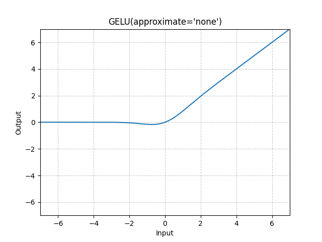
ViTOutput
- Second part of $\text{MLP}$ + optional Dropout
- Second Residual block
1
2
3
4
ViTOutput(
  (dense): Linear(in_features=3072, out_features=768, bias=True)
  (dropout): Dropout(p=0.0, inplace=False)
)
1
2
3
hidden_states = self.dense(hidden_states)
hidden_states = self.dropout(hidden_states)
hidden_states = hidden_states + input_tensor
Classifier
1
Linear(in_features=768, out_features=1000, bias=True)
1
2
3
sequence_output = outputs.last_hidden_state
pooled_output = sequence_output[:, 0, :]
logits = self.classifier(pooled_output)
Loss Function
Task-dependent
| Model | Loss |
|---|---|
| ViT backbone | ❌ none |
| ViTForImageClassification | ✅ CrossEntropy |
| ViTForMaskedImageModeling | ✅ reconstruction loss |
| ViT for detection (DETR-style) | ✅ Hungarian matching + bbox loss |
ViTForMaskedImageModeling
1
2
3
4
(decoder): Sequential(
  (0): Conv2d(768, 768, kernel_size=(1, 1), stride=(1, 1))
  (1): PixelShuffle(upscale_factor=16)
)
Rearranges elements in a tensor of shape $(∗,C×r^2,H,W)$ to a tensor of shape $(∗,C,H×r,W×r)$, where r is an upscale factor.
1
2
3
4
5
6
7
8
9
10
11
12
13
14
15
16
17
18
19
20
21
22
23
24
sequence_output = outputs.last_hidden_state

# Reshape to (batch_size, num_channels, height, width)
sequence_output = sequence_output[:, 1:]
batch_size, sequence_length, num_channels = sequence_output.shape
height = width = math.floor(sequence_length**0.5)
sequence_output = sequence_output.permute(0, 2, 1).reshape(batch_size, num_channels, height, width)

# Reconstruct pixel values
reconstructed_pixel_values = self.decoder(sequence_output)

masked_im_loss = None
if bool_masked_pos is not None:
  size = self.config.image_size // self.config.patch_size
  bool_masked_pos = bool_masked_pos.reshape(-1, size, size)
  mask = (
    bool_masked_pos.repeat_interleave(self.config.patch_size, 1)
    .repeat_interleave(self.config.patch_size, 2)
    .unsqueeze(1)
    .contiguous()
  )
  reconstruction_loss = nn.functional.l1_loss(pixel_values, reconstructed_pixel_values, reduction="none")
  masked_im_loss = (reconstruction_loss * mask).sum() / (mask.sum() + 1e-5) / self.config.num_channels
Hybrid Architecture
As an alternative to raw image patches, the input sequence can be formed from feature maps of a CNN (LeCun et al., 1989). In this hybrid model, the patch embedding projection E (Eq. 1) is applied to patches extracted from a CNN feature map. As a special case, the patches can have spatial size 1x1, which means that the input sequence is obtained by simply flattening the spatial dimensions of the feature map and projecting to the Transformer dimension. The classification input embedding and position embeddings are added as described above.
Fine-Tuning and Higher Resolution
- [[#Optional Interpolation High Resolution]]
Typically, we pre-train ViT on large datasets, and fine-tune to (smaller) downstream tasks. For this, we remove the pre-trained prediction head and attach a zero-initialized D × K feedforward layer, where K is the number of downstream classes.
It is often beneficial to fine-tune at higher resolution than pre-training (Touvron et al., 2019; Kolesnikov et al., 2020). When feeding images of higher resolution, we keep the patch size the same, which results in a larger effective sequence length. The Vision Transformer can handle arbitrary sequence lengths (up to memory constraints), however, the pre-trained position embeddings may no longer be meaningful. We therefore perform 2D interpolation of the pre-trained position embeddings, according to their location in the original image. Note that this resolution adjustment and patch extraction are the only points at which an inductive bias about the 2D structure of the images is manually injected into the Vision Transformer.
Experiments
Dataset
Table are ChatGPT generated
Pre-training Datasets
| Dataset | #Images | #Classes | Purpose | Key Insight |
|---|---|---|---|---|
| ImageNet (ILSVRC-2012) | 1.3M | 1K | Standard training baseline | Small-scale pretraining |
| ImageNet-21k | 14M | 21K | Larger-scale pretraining | More data improves ViT |
| JFT | 303M | 18K | Massive pretraining | Critical for ViT performance |
Downstream (Transfer) Datasets
We de-duplicate the pre-training datasets w.r.t. the test sets of the downstream tasks following Kolesnikov et al. (2020).
| Dataset | Type | Size | Purpose | What it tests |
|---|---|---|---|---|
| ImageNet (val + ReaL) | Natural images | Medium | Evaluation | Label quality & robustness |
| CIFAR-10 | Natural images | Small (32×32) | Transfer | Generalization to small data |
| CIFAR-100 | Natural images | Small | Transfer | Fine-grained classification |
| Oxford-IIIT Pets | Natural images | Small | Transfer | Real-world classification |
| Oxford Flowers-102 | Natural images | Small | Transfer | Fine-grained categories |
VTAB Benchmark (Low-data Transfer)
VTAB evaluates low-data transfer to diverse tasks, using 1000 training examples per task.
| Category | Example Tasks | Data Size | Purpose | What it tests |
|---|---|---|---|---|
| Natural | CIFAR, Pets | 1K samples/task | Low-data transfer | Standard vision tasks |
| Specialized | Medical, Satellite | 1K samples/task | Domain transfer | Out-of-domain generalization |
| Structured | Localization tasks | 1K samples/task | Geometry understanding | Spatial reasoning |
Model Variants
ViT Model Variants
We base ViT configurations on those used for BERT (Devlin et al., 2019), as summarized in Table 1. The “Base” and “Large” models are directly adopted from BERT and we add the larger “Huge” model. In what follows we use brief notation to indicate the model size and the input patch size: for instance, ViT-L/16 means the “Large” variant with 16 × 16 input patch size. Note that the Transformer’s sequence length is inversely proportional to the square of the patch size, thus models with smaller patch size are computationally more expensive.
| Model | Layers | Hidden Size (D) | MLP Size | Heads | Params |
|---|---|---|---|---|---|
| ViT-Base | 12 | 768 | 3072 | 12 | 86M |
| ViT-Large | 24 | 1024 | 4096 | 16 | 307M |
| ViT-Huge | 32 | 1280 | 5120 | 16 | 632M |
Note that the Transformer’s sequence length is inversely proportional to the square of the patch size, thus models with smaller patch size are computationally more expensive.
Sequence length ∝ 1 / (patch size²)
| Patch Size | Sequence Length | Compute Cost | Key Insight |
|---|---|---|---|
| Larger patches (e.g., 32×32) | Shorter sequence | Cheaper | Less detailed |
| Smaller patches (e.g., 16×16, 14×14) | Longer sequence | More expensive | More detailed |
CNN Baseline (ResNet BiT)
For the baseline CNNs, we use ResNet (He et al., 2016), but replace the Batch Normalization layers (Ioffe & Szegedy, 2015) with Group Normalization (Wu & He, 2018), and used standardized convolutions (Qiao et al., 2019). These modifications improve transfer (Kolesnikov et al., 2020), and we denote the modified model “ResNet (BiT)”.
- Standardized Convolution = normalize the convolution weights before applying them
Hybrid Model (CNN + ViT)
For the hybrids, we feed the intermediate feature maps into ViT with patch size of one “pixel”. To experiment with different sequence lengths, we either (i) take the output of stage 4 of a regular ResNet50 or (ii) remove stage 4, place the same number of layers in stage 3 (keeping the total number of layers), and take the output of this extended stage 3. > Option (ii) results in a 4x longer sequence length, and a more expensive ViT model.
| Common Name | Paper Name | Stage Index | Output Stride |
|---|---|---|---|
| Stage 1 | conv2_x | stage 1 | /4 |
| Stage 2 | conv3_x | stage 2 | /8 |
| Stage 3 | conv4_x | stage 3 | /16 |
| Stage 4 | conv5_x | stage 4 | /32 |
Training & Fine-tuning
We train all models, including ResNets, using Adam (Kingma & Ba, 2015) with β1 = 0.9, β2 = 0.999, a batch size of 4096 and apply a high weight decay of 0.1, which we found to be useful for transfer of all models (Appendix D.1 shows that, in contrast to common practices, Adam works slightly better than SGD for ResNets in our setting).
We use a linear learning rate warmup and decay, see Appendix B.1 for details
For fine-tuning we use SGD with momentum, batch size 512, for all models, see Appendix B.1.1.
For ImageNet results in Table 2, we fine-tuned at higher resolution: 512 for ViT-L/16 and 518 for ViT-H/14, and also used Polyak & Juditsky (1992) averaging with a factor of 0.9999 (Ramachandran et al., 2019; Wang et al., 2020b).
Metrics
We report results on downstream datasets either through few-shot or fine-tuning accuracy. Fine-tuning accuracies capture the performance of each model after fine-tuning it on the respective dataset. Few-shot accuracies are obtained by solving a regularized least-squares regression problem that maps the (frozen) representation of a subset of training images to ${−1, 1}^K$ target vectors. This formulation allows us to recover the exact solution in closed form. Though we mainly focus on fine-tuning performance, we sometimes use linear few-shot accuracies for fast on-the-fly evaluation where fine-tuning would be too costly.
References
- Paper: [2010.11929] An Image is Worth 16x16 Words: Transformers for Image Recognition at Scale
- Code: GitHub - google-research/vision_transformer · GitHub
- PyTorch Official:
- HuggingFace:
- Vision Transformer (ViT) Architecture - GeeksforGeeks
- Vision Transformers (ViT) Tutorial: Architecture and Code Examples | DataCamp
- Vision Transformer: What It Is & How It Works [2024 Guide]
- Building a Vision Transformer Model From Scratch | by Matt Nguyen | Toward Humanoids | Medium
- Explaining OpenAI Sora’s Spacetime Patches: The Key Ingredient | Towards Data Science